During machine learning practice or data analysis, when we get a new dataset, what we can do first is to visualize the data to observe how the data distribute and what the relationship between datapoints. We can easily visualize dataset with 2 or 3 variables by plotting 2-demension(2D) or 3-dimension(3D) figure. However, most of the datasets have quite a large number of variables. Therefore it is important to get to know how to visulize high-dimension dataset.
I would like to discuss two popular techniques we usually use for high-dimension dataset visualization: Principal Component Analysis (PCA) and T-distributed Stochastic Neighbor Embedding (t-SNE). We will focus on PCA on this post and more about t-SNE in later post.
What is PCA
PCA tries to out a smaller set of new variables(principal components, PCs) which can capture most of the variation in dataset. We can get some simple examples to make it easy to understand.
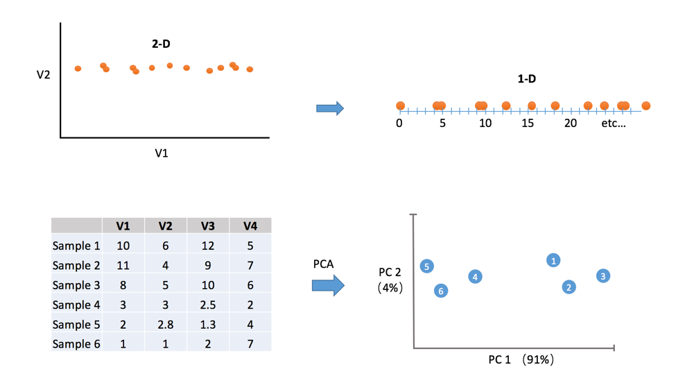 We can observe from the top of Figure 1 that some dimensions may have more important than others. In this case, we can take 2-D data and display it on a 1-D graph without too much information loss. Both graphs say, “the important variation is left to right”. Intuitively, a dimension that has more variability can explain more about the happenings.
We can visulize data with more than 3 variables (in this case is 4 variables) in 2D graph by using PCA…
To describe how the PCA works, we will use two variables simply for convenience. More variables will follow the same way.
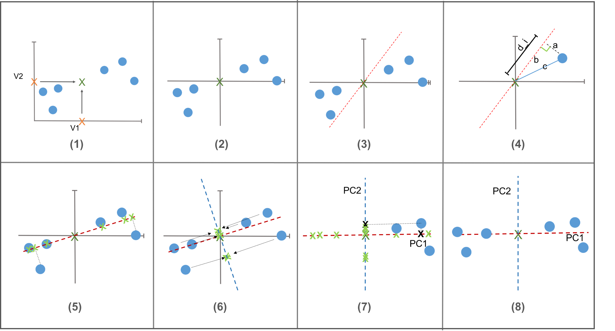
How PCA works
- normalization
- best fitting (projection)
- egienvalue, eigenvector
- loading score, screen plot
Examples
to be continued